Getting started

Jupyter notebook version of this page can be downloaded here.

The latest stable version of PyRigi can be installed by

pip install pyrigi

More detailed installation instructions can be found here.

Once the package is installed, the basic classes Graph and Framework can be imported as follows:

from pyrigi import Graph, Framework

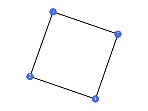
We can specify a graph by its list of edges, see this tutorial for more options.

G = Graph([(0,1), (1,2), (2,3), (0,3)])
G

Graph.from_vertices_and_edges([0, 1, 2, 3], [(0, 1), (0, 3), (1, 2), (2, 3)])

G.plot()

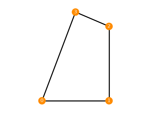
Having graph G, we can construct a framework.

F = Framework(G, {0:[0,0], 1:[1,0], 2:[1,'1/2 * sqrt(5)'], 3:[1/2,'4/3']})
F

Framework(Graph.from_vertices_and_edges([0, 1, 2, 3], [(0, 1), (0, 3), (1, 2), (2, 3)]), {0: ['0', '0'], 1: ['1', '0'], 2: ['1', 'sqrt(5)/2'], 3: ['0.500000000000000', '4/3']})

Notice that in order to keep the coordinates symbolic, they must be entered as strings (or SymPy expressions).

We can plot frameworks and graphs, see also the Plotting tutorial.

F.plot()

Positions of vertices can be read using square brackets:

F[2]

\[\begin{split}\displaystyle \left[\begin{matrix}1\\\frac{\sqrt{5}}{2}\end{matrix}\right]\end{split}\]

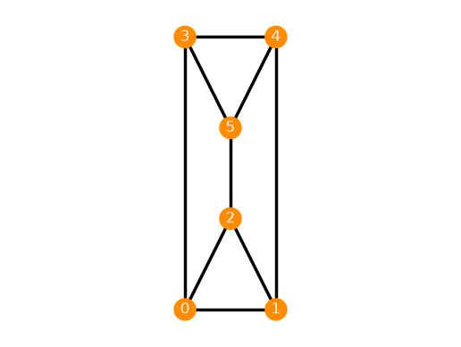
There are also some predefined graphs and frameworks, see graphDB and frameworkDB (also this tutorial)

import pyrigi.frameworkDB as frameworks

TP_inf_flex = frameworks.ThreePrism('parallel')
TP_inf_flex.plot()

There is also a possibility to draw a graph using mouse.

Rigidity properties

Various rigidity properties can be checked by calling class methods, some examples are below. See also this tutorial.

Infinitesimal rigidity

The framework of 3-prism created above is infinitesimally flexible.

TP_inf_flex.is_inf_rigid()

False

It has the following rigidity matrix:

TP_inf_flex.rigidity_matrix()

\[\begin{split}\displaystyle \left[\begin{array}{cccccccccccc}-2 & 0 & 2 & 0 & 0 & 0 & 0 & 0 & 0 & 0 & 0 & 0\\-1 & -2 & 0 & 0 & 1 & 2 & 0 & 0 & 0 & 0 & 0 & 0\\0 & -6 & 0 & 0 & 0 & 0 & 0 & 6 & 0 & 0 & 0 & 0\\0 & 0 & 1 & -2 & -1 & 2 & 0 & 0 & 0 & 0 & 0 & 0\\0 & 0 & 0 & -6 & 0 & 0 & 0 & 0 & 0 & 6 & 0 & 0\\0 & 0 & 0 & 0 & 0 & -2 & 0 & 0 & 0 & 0 & 0 & 2\\0 & 0 & 0 & 0 & 0 & 0 & -2 & 0 & 2 & 0 & 0 & 0\\0 & 0 & 0 & 0 & 0 & 0 & -1 & 2 & 0 & 0 & 1 & -2\\0 & 0 & 0 & 0 & 0 & 0 & 0 & 0 & 1 & 2 & -1 & -2\end{array}\right]\end{split}\]

The space of nontrivial infinitesimal flexes is generated by:

TP_inf_flex.nontrivial_inf_flexes()

[Matrix([
 [1],
 [0],
 [1],
 [0],
 [1],
 [0],
 [0],
 [0],
 [0],
 [0],
 [0],
 [0]])]

Generic rigidity

Now we retrieve the underlying graph and check that it is (generically) 2-rigid.

G_TP = TP_inf_flex.graph
G_TP.is_rigid()

True

It is also (generically) 1-rigid.

G_TP.is_rigid(dim=1)

True

No combinatorial characterization is known for 3-rigidity, but a randomized algorithm can be used based on Theorem 4.

G_TP.is_rigid(dim=3, algorithm="randomized")

False

We can check also {prf:ref}`global <def-globally-rigid-graph>` or {prf:ref}`redundant <def-redundantly-rigid-graph>` rigidity:

G_TP.is_globally_rigid()

False

G_TP.is_redundantly_rigid()

False