Plotting
This notebook can be downloaded here.
import pyrigi.frameworkDB as frameworks
import pyrigi.graphDB as graphs
from pyrigi import Graph, Framework
Methods Graph.plot() and Framework.plot() offer various plotting options.
The default behaviour is the following:
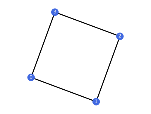
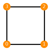
G = Graph([(0,1), (1,2), (2,3), (0,3)])
G.plot()
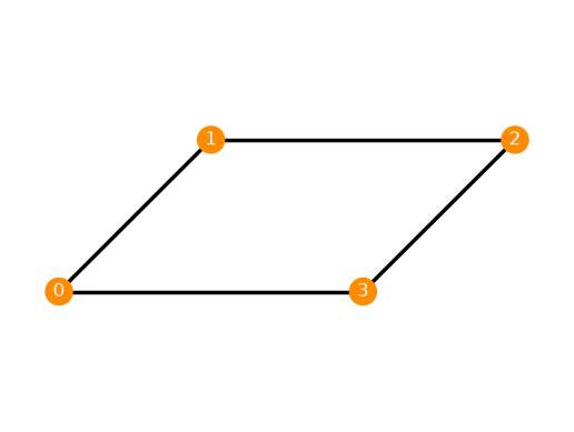
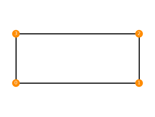
F = Framework(G, {0: (0,0), 1: (1,1), 2: (3,1), 3: (2,0)})
F.plot()
Graph layouts
By default, a placement is generated using spring_layout().
G = graphs.ThreePrism()
G.plot()
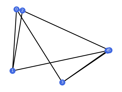
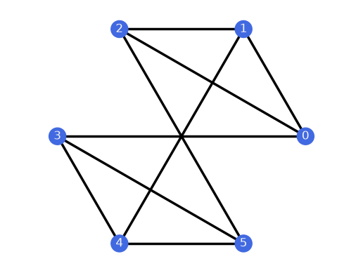
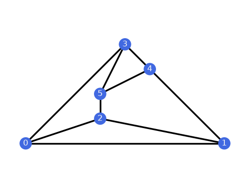
Other options use random_layout(), circular_layout() or planar_layout():
G.plot(layout="random")
G.plot(layout="circular")
G.plot(layout="planar")
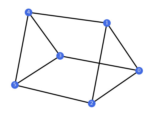
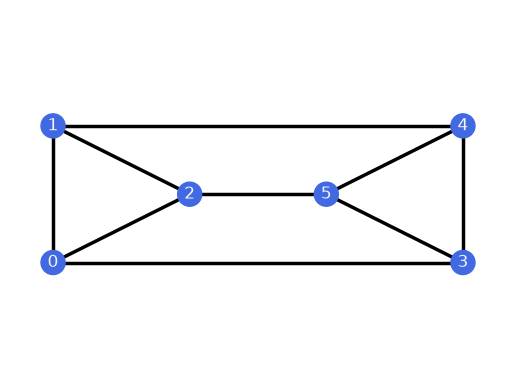
One can also specify a placement of the vertices explicitly:
G.plot(placement={0: (0, 0), 1: (0, 2), 2: (2, 1), 3: (6, 0), 4: (6, 2), 5: (4, 1)})
Canvas options
The size of the canvas can be specified.
Square = frameworks.Square()
Square.plot(canvas_width=2)
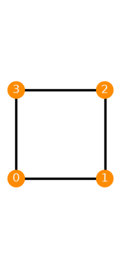
Square.plot(canvas_height=2)

Square.plot(canvas_width=2, canvas_height=2)
Also the aspect ratio:
Square.plot(aspect_ratio=0.4)
Formatting
There are various options to format a plot. One can pass them as keywords arguments, for instance vertex color/size or label color/size can be changed.
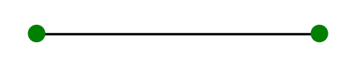
G = Graph([[0,1]])
realization = {0: [0,0], 1: [1,0]}
G.plot(placement=realization, canvas_height=1, vertex_labels=False, vertex_color='green')
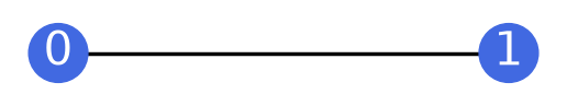
G.plot(placement=realization, canvas_height=1, vertex_size=1500, font_size=30, font_color='#FFFFFF')
In order to format multiple plots using the same arguments,
we can create an instance of class PlotStyle (see also PlotStyle2D)
and pass it to each plot.
from pyrigi import PlotStyle
plot_style = PlotStyle(
canvas_height=1,
vertex_color='blue',
vertex_labels=False,
)
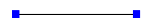
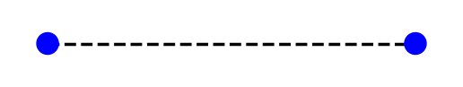
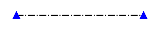
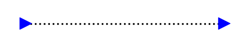
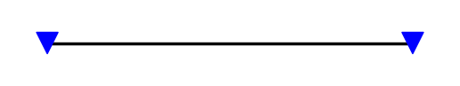
There are various styles of vertices and edges.
G.plot(plot_style, placement=realization, vertex_shape='s', edge_style='-')
G.plot(plot_style, placement=realization, vertex_shape='o', edge_style='--')
G.plot(plot_style, placement=realization, vertex_shape='^', edge_style='-.')
G.plot(plot_style, placement=realization, vertex_shape='>', edge_style=':')
G.plot(plot_style, placement=realization, vertex_shape='v', edge_style='solid')
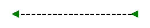
We can also change some values of plot_style in two different ways.
The first is using method PlotStyle.update().
plot_style.update(vertex_color='green')
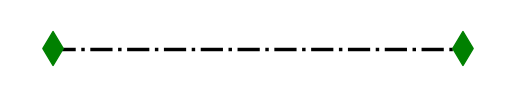
G.plot(plot_style, placement=realization, vertex_shape='<', edge_style='dashed')
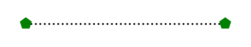
G.plot(plot_style, placement=realization, vertex_shape='d', edge_style='dashdot')
G.plot(plot_style, placement=realization, vertex_shape='p', edge_style='dotted')
The second is a direct assignment to an attribute.
plot_style.vertex_shape = 'h'
G.plot(plot_style, placement=realization, edge_width=3)
plot_style.vertex_shape = '8'
G.plot(plot_style, placement=realization, edge_width=5)

Edge coloring
The color of all edges can be changed.
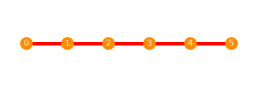
P = graphs.Path(6)
plot_style = PlotStyle(
canvas_height=2,
edge_width=5,
)
realization = {v: [v, 0] for v in P.vertex_list()}
P.plot(plot_style, placement=realization, edge_color='red')
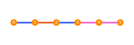
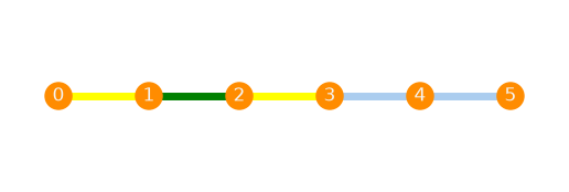
If a partition of the edges is specified, then each part is colored differently.
P.plot(plot_style, placement=realization, edge_colors_custom=[[[0, 1], [2, 3]], [[1, 2]], [[5, 4], [4, 3]]])
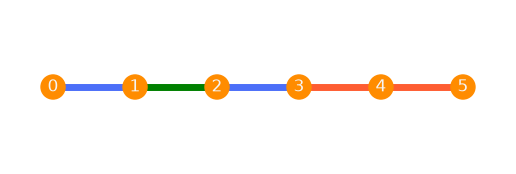
If the partition is incomplete, the missing edges get PlotStyle.edge_color.
plot_style.update(edge_color='green')
P.plot(plot_style, placement=realization, edge_colors_custom=[[[0, 1], [2, 3]], [[5, 4], [4, 3]]])
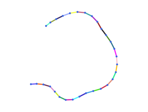
Visually distinct colors are generated using the package distinctipy.
P30 = graphs.Path(30)
P30.plot(
vertex_size=15,
vertex_labels=False,
edge_colors_custom=[[e] for e in P30.edge_list()],
edge_width=3
)
Another possibility is to provide a dictionary assigning to a color a list of edges.
Missing edges again get PlotStyle.edge_color.
P.plot(plot_style,
placement=realization,
edge_colors_custom={
"yellow": [[0, 1], [2, 3]],
"#ABCDEF": [[5, 4], [4, 3]]
},
)
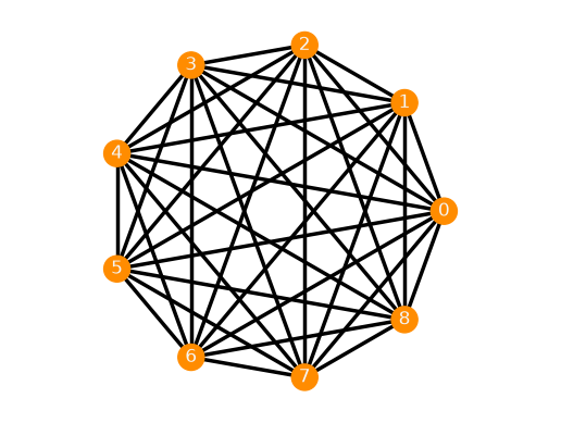
Framework plotting
Currently, only plots of frameworks in the plane are implemented.
F = frameworks.Complete(9)
F.plot()
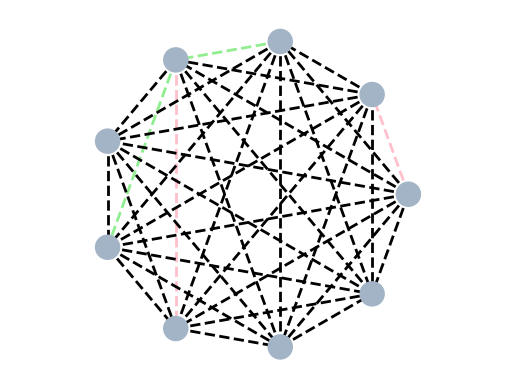
The same formatting options as for graphs are available for frameworks.
See also PlotStyle2D and PlotStyle3D.
F = frameworks.Complete(9)
F.plot(
vertex_labels=False,
vertex_color='#A2B4C6',
edge_style='dashed',
edge_width=2,
edge_colors_custom={"pink": [[0,1],[3,6]], "lightgreen": [[2, 3], [3, 5]]}
)
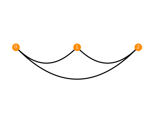
Collinear Configurations
For collinear configurations and frameworks in \(\RR\), the edges are automatically visualized as arcs in \(\RR^2\)
F = Framework.Complete([[0],[1],[2]])
F.plot()
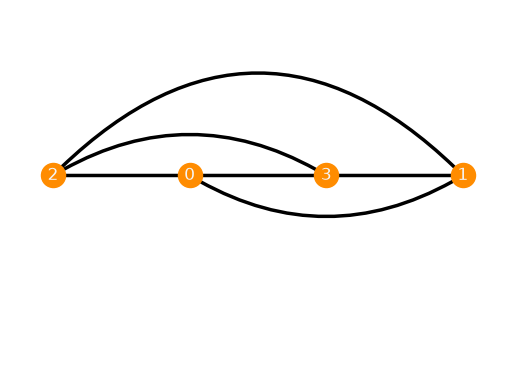
Using the keyword arc_angles_dict, we are able to specify the pitch of the individual arcs. This parameter can be specified in
radians as a float if the same pitch for every arc is desired and a list[float] or a
dict[Edge, float] if the pitch is supposed to be provided for each arc individually.
F = Framework.Complete([[1],[3],[0],[2]])
F.plot(arc_angles_dict={(0,1):0.3, (0,2):0, (0,3):0, (1,2):0.5, (1,3):0, (2,3):-0.3})
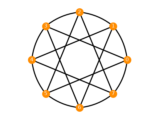
We can also enhance the visualization of other configurations using the
boolean edges_as_arcs. This is particularly useful for visualizing almost or piecewise
collinear configurations, but of course, it can also be applied to arbitrary frameworks.
It is possible have fewer edges in the dict; the remaining edges are than padded with
the default value arc_angle=math.pi/6. Here, we want to have some straight edges, so we
redefine the arc_angle as \(0\).
F = frameworks.CnSymmetricFourRegular(n=8)
F.plot(edges_as_arcs=True, arc_angle=0, arc_angles_dict={(i,i+1):0.15 for i in range(7)} | {(0,7):-0.15})
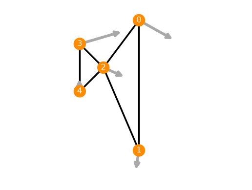
Infinitesimal Flexes
It is possible to include infinitesimal flexes in the plot. With the keyword
inf_flex=n, we can pick the n-th nontrivial infinitesimal flex from
a basis of the rigidity matrix’s kernel. There are several keywords that allow
us to alter the style of the drawn arrows. A full list of the optional plotting
parameters can be found in the API reference: PlotStyle.
G = Graph([[0, 1], [0, 2], [1, 2], [2, 3], [2, 4], [3, 4]])
realization = {0: [6, 8], 1: [6, -14], 2: [0, 0], 3: [-4, 4], 4: [-4, -4]}
F = Framework(G, realization)
F.plot(
inf_flex=0,
flex_width=4,
flex_length=0.25,
flex_color="darkgrey",
flex_style="-",
flex_arrow_size=15
)
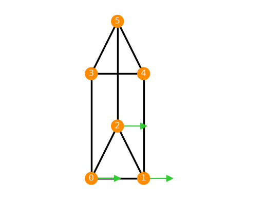
It is also possible to provide a specific infinitesimal flex with the following chain of commands:
F = frameworks.ThreePrism(realization="flexible")
inf_flex = F.nontrivial_inf_flexes()[0]
F.plot(inf_flex=inf_flex)
It is important to use the same order of the vertices of F as Graph.vertex_list() when
providing the infinitesimal flex as a Matrix. To circumvent that,
we also support adding an infinitesimal flex as a Dict[Vertex, Sequence[Number]].
In both of the cases where the user provides an infinitesimal flex, it is
internally checked whether the provided vector lies in the kernel of the rigidity matrix.
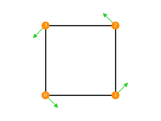
F = frameworks.Square()
inf_flex = {0: (1, -1), 1: (1, 1), 2: (-1, 1), 3: (-1, -1)}
F.plot(inf_flex=inf_flex)
Equilibrium Stresses
We can also plot stresses. Contrary to flexes, stresses exist as edge labels.
Analogous to the way that infinitesimal flexes can be visualized (see the previous
section), a stress can be provided either as the n-th equilibrium stress, as a
specific stress given by a Matrix or alternatively as a dict[Edge, Number].
It is internally checked, whether the provided stress lies in the cokernel of the
rigidity matrix. We can specify the positions of the stress labels using the keyword
stress_label_pos, which can either be set for all edges as the same float from \([0,1]\)
or individually using a dict[DirectedEdge, float]. This float specifies the position on
the line segment given by the edges. The missing edges labels are automatically
centered on the edge. A full list of the optional plotting parameters can be found in
the API reference: PlotStyle.
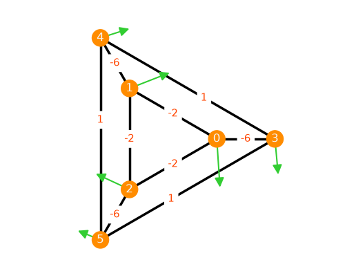
F = frameworks.Frustum(3)
F.plot(
inf_flex=0,
stress=0,
stress_color = "orangered",
stress_fontsize = 11,
stress_label_positions = {(3,5): 0.6, (3,4):0.4, (4,5):0.4},
stress_rotate_labels = False
)
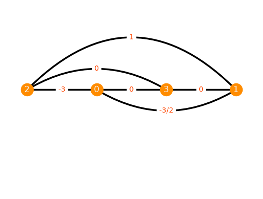
The visualization of equilibrium stresses can be combined with the plotting of collinear configurations from a previous section that displays edges as curved arcs.
F = Framework.Complete([[1],[3],[0],[2]])
F.plot(stress=0, arc_angles_dict={(0,1):0.3, (0,2):0, (0,3):0, (1,2):0.5, (1,3):0, (2,3):-0.3})
Plotting in 3 Dimensions
Plotting in 3 dimensions is also possible. The plot can be made interactive by using cell magic:
%matplotlib widget
Using the keyword axis_scales, we can decide whether we want to avoid stretching the framework ((1,1,1))
or whether we want to transform the framework to a different aspect ratio.
The other possible keywords can be found in the corresponding API reference: plot3D().
F = frameworks.Complete(4, dim=3)
F.plot3D()
In addition, it is possible to animate a rotation sequence around a specified axis:
G = graphs.DoubleBanana()
F = Framework(G, realization={0:(0,0,-2), 1:(0,0,3), 2:(1.25,1,0.5), 3:(1.25,-1,0.5), 4:(3,0,0.5),
5:(-1.25,-1,0.5), 6:(-1.2,1,0.5), 7:(-3,0,0.5)})
F.animate3D_rotation(rotation_axis=[0,0,1], axis_scales=(1,1,1))
We can return to the usual inline mode using the command %matplotlib inline.
Note that triggering this command after using %matplotlib widget
may cause the jupyter notebook to render additional pictures.
If this behavior is undesirable, we suggest reevaluating the affected cells.
It is also possible to plot infinitesimal flexes and equilibrium stresses in 3D using the
inf_flex and stress keywords, respectively. For details, the entire list of parameters
concerning infinitesimal flexes and equilibrium stresses can
be looked up in the corresponding API reference: PlotStyle.
F = frameworks.Octahedron(realization="Bricard_plane")
F.plot(inf_flex=0,
stress=0,
flex_length=0.25,
stress_fontsize=11,
axis_scales=(0.625,0.625,0.625),
stress_label_positions={e: 0.6 for e in F.graph.edges}
)